Dynamical Systems#
DynamicalSystem is the class used in Siconos to describe a set of ordinary differential equations, which is the essential first step of any nonsmooth problem description in Siconos.
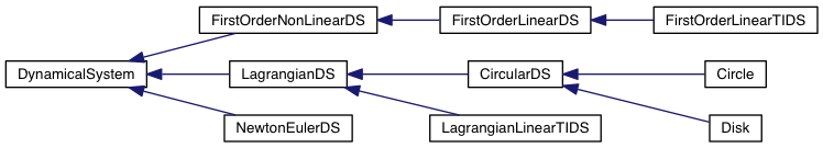
This base class defines a common interface to all systems. To fit with different types of problems, we propose several derived classes representing some specific formulations, as described below.
As usual, a complete description of the interface (members and methods) of these classes can be found in the doxygen documentation, see for example DynamicalSystem.
Note that DynamicalSystem is an abstract class, and no object of this type can be implemented. It just provides a generic interface for all systems.
Overview#
The most general way to write dynamical systems in Siconos is
n-dimensional set of equations where
t is the time
\(x \in R^{n}\) is the state.
\(\dot x\) the derivative of the state according to time
\(z \in R^{s}\) is a vector of arbitrary algebraic variables, some sort of discrete state. For example, z may be used to set some perturbation parameters, or anything else.
\(g : \mathbb{R}^{n} \times \mathbb{R}^n \times \mathbb{R} \times \mathbb{R}^s \to \mathbb{R}^{n}\).
Under some specific conditions, we can rewrite this as:
“rhs” means right-hand side. Note that in that case \(\nabla_{\dot x} g\) must be invertible.
The aim of this class is to provide some members and functions for all dynamical systems types (ie for all derived classes), but with some specific behaviors depending on the type of system (see the related sections below for details).
That means that all members and functions described below are also available in any of the derived classes.
Each system is identified thanks to a number and the current state of the system is saved as a vector DynamicalSystem::x(), with x[0]= \(x\) and x[1]= \(\dot x\).
All the functions and their gradients ( \(g, rhs, \nabla_x g\) …) can be accessed with functions like DynamicalSystem::jacobianRhsx() for \(\nabla_{x} rhs(x, t, z)\). Check the reference for a complete list of the members and methods.
The common rules for all members are, ‘name’ being the required variable:
getName() to get a copy of the content of the object
name() to get a pointer to the object
setName(obj) to copy obj into Name
setNamePtr(objPtr) to link objPtr with Name
Plug-in: some members can be connected to user plug-in functions, used to compute them. In that case, the following methods can be used: - setComputeNameFunction(…) to link name with your own function * computeName(…) to compute name using your own function
For details about plug-in mechanism, see User-defined plugins.
For instance, if you want to use the internal forces operators in Lagrangian systems (see below), two solutions: either the forces are a constant vector or are connected to a plug-in and can then depend on time, state of the system …
First case:
// we suppose that ds is an existing pointer to a LagrangianDS
SP::SiconosMatrix myF(new SimpleVector(3));
// fill my G in ...
ds->setFInt(*myF); // copy myF values into fInt
// OR
// link fInt to myF: any change in one of them will impact on the other.
ds->setFIntPtr(myF);
Second case:
// we suppose that ds is an existing pointer to a LagrangianDS
// and that myFunction is a c function implemented in myPlugin.cpp
ds->setComputeFInt("myPlugin", "myFunction");
// ...
ds->computeFInt(time);
// compute fInt value at time for the current state
Note that the signature (e ie the number and type of arguments) of the function you use in your plugin must be exactly the same as the one given in kernel/src/plugin/DefaultPlugin.cpp for the corresponding function.
Common interface#
The following functions are (and must) be present in any class derived from DynamicalSystems
First order dynamical systems#
Non linear#
They are described by the following set:
with:
\(M \in \mathbb{R}^{n \times n}\)
f(x,t): the vector field - \(f: \mathbb{R}^{n} \times \mathbb{R} \to \mathbb{R}^n\)
r: input due to non-smooth behavior - Vector of size n.
JacobianXF = \(\nabla_x f(t,x,z)\), a nX n square matrix, is also a member of the class.
M is supposed to be invertible (if not, we can not compute x[1]=rhs …).
initial conditions are given by the member x0, vector of size n. This corresponds to x value when simulation is starting, e ie after a call to simulation initialize() function. n
There are plug-in functions in this class for f and its Jacobian, jacobianfx.
We have:
g and its gradients
Linear#
Described by the set of n equations and initial conditions:
With:
A(t,z): nXn matrix, state independent but possibly time-dependent.
b(t,z): Vector of size n, possibly time-dependent. A and B have corresponding plug-in functions. Other variables are those of
DynamicalSystemand FirstOrderNonLinearDS classes, but some of them are not defined and thus not usable: ng and its gradients
f and its gradient
And we have:
Linear and time-invariant#
class FirstOrderLinearTIDS
Derived from FirstOrderLinearDS, described by the set of n equations and initial conditions:
Same as for FirstOrderLinearDS but with A and b constant (ie no plug-in).
Second order (Lagrangian) systems#
Non linear#
LagrangianDS, derived from DynamicalSystem.
Lagrangian second order non linear systems are described by the following set of nDof equations + initial conditions:
with:
Mass(q,z): nDofX nDof matrix of inertia.
q: state of the system - Vector of size nDof.
\(\dot q\) the derivative of the state according to time.
\(f_L(t,\dot q , q , z) = F_{Ext}(t,z) - fGyr(\dot q, q,z) - F_{Int}(t,\dot q , q , z)\)
\(fGyr(\dot q, q,z)\): non linear terms, time-independent - Vector of size nDof.
\(F_{Int}(t,\dot q , q , z)\): time-dependent linear terms - Vector of size nDof.
\(F_{Ext}(t,z)\): external forces, time-dependent BUT do not depend on state - Vector of size nDof.
p: input due to non-smooth behavior - Vector of size nDof.
Note that the decomposition of \(f_L\) is just there to propose a more “comfortable” interface for user but does not interfer with simulation process.
Some gradients are also required:
jacobianFInt[0] = \(\nabla_q F_{Int}(t,q,\dot q,z)\) - nDofX nDof matrix.
jacobianFInt[1] = \(\nabla_{\dot q} F_{Int}(t,q,\dot q,z)\) - nDof X nDof matrix.
jacobianfGyr[0] = \(\nabla_q fGyr(\dot q, q, z)\) - nDof X nDof matrix.
jacobianfGyr[1] = \(\nabla_{\dot q}fGyr(\dot q, q, z)\) - nDof X nDof matrix.
We consider that the Mass matrix is invertible and that its gradient is null.
There are plug-in functions in this class for \(F_{int}, F_{Ext}, M, fGyr\) and the four Jacobian matrices.
Other variables are those of DynamicalSystem class, but some of them are not defined and thus not usable: n
* g and its gradients
Links with DynamicalSystem are, \(n= 2 ndof\) and \(x = \left[\begin{array}{c}q \\ \dot q\end{array}\right]\). n
And we have:
I: identity matrix.
Linear and time-invariant#
class LagrangianLinearTIDS, derived from LagrangianDS.
With:
C: constant viscosity nDof X nDof matrix
K: constant rigidity nDof X nDof matrix
Other variables are those of DynamicalSystem and LagrangianDS classes, but some of them are not defined and thus not usable: n
* g and its gradients
* fL, fInt, fGyr and their gradients.
And we have:
Dynamical Systems plug-in functions#
DynamicalSystem: \(g(t,\dot x,x,z), \ \ \nabla_x g(t,\dot x,x,z), \ \ \nabla_{\dot x} g(t,\dot x,x,z)\)FirstOrderNonLinearDS: \(f(t,x,z), \ \ \nabla_x f(t,x,z)\)FirstOrderLinearDS: A(t,z), b(t,z)LagrangianDS: \(M(q,z), \ \ fGyr(\dot q,q,z), \ \ F_{Int}(t,\dot q,q ,z), \ \ F_{Ext}(t,z), \ \ \nabla_q F_{Int}(t,\dot q,q,z), \ \ \nabla_{\dot q}F_{Int}(t,\dot q, q, z), \ \ \nabla_q fGyr(\dot q, q, z), \ \ \nabla_{\dot q}fGyr(\dot q, q, z)\).LagrangianLinearTIDS: \(F_{Ext}(t,z)\)