Tutorial : a column of three beads#
This tutorial deals with a column of beads, subjected to the gravity. It introduces Lagrangian Linear systems with Lagrangian Linear Relations and Newton impact law.
Building the Non-Smooth Dynamical System#
As described in the figure below, we consider a ball of mass \(m\) and radius \(R\), described by 3 generalized coordinates \(q=(z,x,\theta)\) The ball is subjected to the gravity \(g\). The system is also constituted by a rigid plane, defined by its position \(h\) with respect to the axis Oz. We assume that the position of the plane is fixed and not modeled as a dynamical system.

fig 1: Coordinate system#
The equation of motion of a ball is given by
with
\(M\) the inertia term, a \(n\times{}n\) matrix.
\(p\) the force due to the non-smooth law, ie the reaction at impact.
\(F_{ext}(t): \mathcal R \rightarrow \mathcal R^{n}\) the given external force.
That fits with Lagrangian, Linear and Time-Invariant Dynamical System, represented by LagrangianLinearTIDS class (see ref dsInSiconos).
Next, we will suppose that we have a column of “dsNumber” balls like the one above (mass and radius may be different, and if necessary, variables will be indexed by \(i\), the number of the ball). Each ball is governed by a linear system like the one written for a single ball and may be in contact with the balls above and below it.
Let us now start the writing of the input file. Like for the first tutorial, we create a new directory, multiBeads, and save the template given ref tutGCtemplate “here” as multiBeads.cpp.
We start by setting some parameters, like the number of balls, their initial positions and velocities and so on:
// User-defined main parameters
unsigned int dsNumber = 10;      // the number of dynamical systems
unsigned int nDof = 3;           // degrees of freedom for beads
double increment_position = 1;   // initial position increment from one DS to the following
double increment_velocity = 0;   // initial velocity increment from one DS to the following
double t0 = 0;                   // initial computation time
double T = 10;                   // final computation time
double h = 0.005;                // time step
double position_init = 10.5;     // initial position for lowest bead.
double velocity_init = 0.0;      // initial velocity for lowest bead.
double R = 0.1;                  // balls radius
Then, we define some initial conditions for the balls, and create the corresponding Dynamical Systems, all of type Lagrangian, Linear and Time Invariant.
All the systems are inserted in a container, a DynamicalSystemsSet, named allDS.
From now on, to simplify writing, we suppose that all balls have the same mass, \(m = 1\), and the same radius, \(R=0.1\):
// -------------------------
// --- Dynamical systems ---
// -------------------------

// mass matrix, set to identity
SP::SiconosMatrix Mass = new SimpleMatrix(nDof,nDof);
Mass->eye();
(*Mass)(2,2) = 3.0/5*R*R;

// -- Initial positions and velocities --
// q0[i] and v0[i] correspond to position and velocity of ball i.
vector<SimpleVector *> q0;
vector<SimpleVector *> v0;
q0.resize(dsNumber,NULL);
v0.resize(dsNumber,NULL);

for (unsigned i = 0; i < dsNumber; ++i)
{
    // Memory allocation for q0[i] and v0[i]
    q0[i] = new SimpleVector(nDof);
    v0[i] = new SimpleVector(nDof);
    // set values
    (*(q0[i]))(0) = position_init;
    (*(v0[i]))(0) = velocity_init;
    // Create a new Lagrangian Linear Dynamical System, with q0] and v0[i] as initial conditions,
    // Mass as mass matrix and i as number of identification.
    // The system is then inserted in allDS.
    allDS.insert( new LagrangianLinearTIDS(i,nDof,*(q0[i]),*(v0[i]),*Mass));
    // Increment values for next system
    position_init+= increment_position;
    velocity_init+= increment_velocity;
}
Next, it is necessary to define the external forces, the gravity, applied on each ball. According to Dynamical Systems plug-in functions, a plug-in function is available for those forces. (For details on plug-in functions, see User-defined plugins). Its signature (the type of its arguments) is given in DefaultPlugin.cpp. So we copy it in a new file, say BeadsPlugin.cpp, and we define an extern function, gravity.:
const double m = 1; // bead mass
const double g = 9.81; // gravity
extern "C" void gravity(unsigned int sizeOfq, double time,    double * fExt, double *param)
{
    // set fExt components to 0
    for (unsigned int i = 0; i < sizeOfq; i++)
    fExt[i] = 0.0;
    // apply gravity
    fExt[0] = -m*g;
}
Warning
gravity must be an extern “C” function, and code is C, not C++.
the name of the plugin file, BeadsPlugin.cpp here, must be xxxPlugin.cpp, xxx being whatever you want.
Now we have to say “use gravity from BeadsPlugin.cpp to compute the external forces of my systems.” This is done thanks to “setComputeFExtFunction” function, in multiBeads.cpp:
//
CheckInsertDS checkDS;
for (i=0;i<dsNumber;i++)
   {
     // Memory allocation for q0[i] and v0[i]
     q0[i] = new SimpleVector(nDof);
     v0[i] = new SimpleVector(nDof);
     // set values
     (*(q0[i]))(0) = position_init;
     (*(v0[i]))(0) = velocity_init;
     // Create and insert in allDS a new Lagrangian Linear Dynamical System ...
     checkDS = allDS.insert(new LagrangianLinearTIDS(i,nDof,*(q0[i]),*(v0[i]),*Mass));
     // Note that we now use a CheckInsertDS object: checkDS.first is
     // an iterator that points to the DS inserted above.
     //
     // Set the external forces for the last created system.
     (static_cast<LagrangianDS*>(*(checkDS.first)))->setComputeFExtFunction("BeadsPlugin.so", "gravity");
     // A cast is required, since allDS handles DynamicalSystem*,
     // not LagrangianLinearTIDS*.
     // Increment values for next system
     position_init+= increment_position;
     velocity_init+= increment_velocity;
   }
From this point, any call to the external forces of a system in allDS will result in a call to the function gravity defined in BeadsPlugin.cpp.
Remark: \(m\) and \(R\) are set inside the BeadsPlugin file but it would also be possible, and maybe better, to pass them as parameters in gravity function. See ref doc_usingPlugin for details on that option.
Ok, now DynamicalSystems are clearly defined and all saved in allDS. Let’s turn our attention to Interactions. In the same way, they will be handled by a container, an InteractionsSet, named allInteractions. The potential interactions are the contacts between beads and the impact on the ground. Thus, for dsNumbers systems, there are dsNumbers-1 “bead-bead” Interactions plus one between the “bottom bead” and the floor.
We start with bead-floor Interaction: the ball at the bottom bounces on the rigid plane, introducing a constraint on the position of the ball, given by: \(z-R-h\geq 0\). To define an Interaction, it is first necessary to set some relations between local variables at contact and the global coordinates. Thus, as a local variables of the Interaction, we introduce \(y\) as the distance between the ball and the floor and \(\lambda\) as the multiplier that corresponds to the reaction at contact. Then the relation is written,
(next, we set h=0).
Finally we need to define a non-smooth law to define the behavior of the ball at impact. The unilateral constraint is such that
completed with a Newton Impact law, for which we set the restitutive coefficient \(e\) to 0.9:
with \(t^+\) and \(t^-\) being post and pre-impact times.
The first Interaction can then be constructed:
// -------------------
// --- Interactions---
// -------------------
InteractionsSet allInteractions;
// The total number of Interactions
int interactionNumber = dsNumber;
// Interaction first bead and floor
// A set for the systems handles by the "current" Interaction
DynamicalSystemsSet dsConcerned;
// Only the "bottom" bead is concerned by this first Interaction,
// therefore DynamicalSystem number 0.
dsConcerned.insert(allDS.getDynamicalSystemPtr(0));
// -- Newton impact law --
double e = 0.9;
NonSmoothLaw * nslaw0 = new NewtonImpactNSL(e);
// Lagrangian Relation
unsigned int interactionSize = 1; // y vector size
SiconosMatrix *H = new SimpleMatrix(interactionSize,nDof);
(*H)(0,0) = 1.0;
SiconosVector *b = new SimpleVector(interactionSize);
(*b)(0) = -R;
Relation * relation0 = new LagrangianLinearR(*H,*b);
// Interaction
unsigned int num = 0 ; // an id number for the Interaction
Interaction * inter0 = new Interaction("bead-floor", dsConcerned,num,interactionSize, nslaw0, relation0);
allInteractions.insert(inter0);
In the same way, the potential contact between two balls introduces some new constraints:
\((z_i-R_i)-(z_j-R_j)-h \geq 0\), if ball \(i\) is on top of ball \(j\).
So if we consider the Interaction between ball \(i\) and \(j\), \(y\) being the distance between two balls and \(\lambda\) the multiplier, we get:
With the same non smooth law as for the first Interaction:
// A list of names for the Interactions
vector<string> id;
id.resize(interactionNumber-1);
CheckInsertInteraction checkInter;
// A vector that will handle all the relations
vector<Relation*> LLR(interactionNumber-1);
//
SiconosMatrix *H1 = new SimpleMatrix(1,2*nDof);
if (dsNumber>1)
{
    (*H1)(0,0) = -1.0;
    (*H1)(0,3) = 1.0;
    // Since Ri=Rj and h=0, we do not need to set b.
    Relation * relation = new LagrangianLinearR(*H1);
    for (i=1;(int)i<interactionNumber;i++)
    {
        // The systems handled by the current Interaction ...
        dsConcerned.clear();
        dsConcerned.insert(allDS.getDynamicalSystemPtr(i-1));
        dsConcerned.insert(allDS.getDynamicalSystemPtr(i));
        // The id: "i"
        ostringstream ostr;
        ostr << i;
        id[i-1]= ostr.str();
        // The relations
        LLR[i-1] = new LagrangianLinearR(*relation); // we use copy constructor to built all relations
        checkInter = allInteractions.insert( new Interaction(id[i-1], dsConcerned,i,interactionSize, nslaw0, LLR[i-1]));
    }
    delete relation;
}
Note that each Relation corresponds to one and only one Interaction (which is not the case of NonSmoothLaw); that’s why we need to built a new Relation LLR[i-1] for each Interaction.
Everything is now ready to build the NonSmoothDynamicalSystem and the related Model:
// --------------------------------
// --- NonSmoothDynamicalSystem ---
// --------------------------------
NonSmoothDynamicalSystem * nsds = new NonSmoothDynamicalSystem(allDS, allInteractions);
// -------------
// --- Model ---
// -------------
Model * multiBeads = new Model(t0,T);
multiBeads->setNonSmoothDynamicalSystemPtr(nsds); // set NonSmoothDynamicalSystem of this model
The Simulation#
Time-Stepping scheme#
As a first example, we will use a Moreau’s time-stepping scheme, where the non-smooth problem will be written as a LCP. The process is more or less the same as for the Diode Bridge case, so we won’t detail it. The only difference is that now, the OneStepIntegrator handles several DynamicalSystems:
string solverName = "Lemke";      // solver algorithm used for non-smooth problem
Simulation* s = new TimeStepping(multiBeads);
// -- Time discretisation --
TimeDiscretisation * t = new TimeDiscretisation(h,s);
// -- OneStepIntegrators --
double theta = 0.5000001;
OneStepIntegrator * OSI = new Moreau(allDS , theta ,s);
// That means that all systems in allDS have the same theta value.
// -- OneStepNsProblem --
OneStepNSProblem * osnspb = new LCP(s,"LCP",solverName,10001, 0.001);
Event-Driven algorithm#
In that second part, an event-driven algorithm is used to solve the problem. Event-Driven Simulation principle is detailed in Event-Driven schemes.
The dynamics is decomposed in “modes”, time-intervalls where the dynamics is smooth and discrete events where the dynamics is non-smooth.
In the present case, non smooth events will corresponds to impacts between balls. Each time such an event is detected, a non-smooth problem is formalized and solved (as a LCP here) while between events, the systems are integrated thanks to Lsodar, ODE solver with roots-finding algorithm.
As for the Time-stepping, we first need to built the simulation and then its time-discretisation:
// The simulation belongs to Model multiBeads
EventDriven* s = new EventDriven(multiBeads);
TimeDiscretisation * t = new TimeDiscretisation(h,s);
Next step is the declaration of integrators for the dynamical systems. The integrator will handle all the DynamicalSystems of the Model. During integration of the systems, Lsodar will search for roots of some equations (the constraints ie the Interactions of the NonSmoothDynamicalSystem). The required OSI type is Lsodar, applied to allDS:
OneStepIntegrator * OSI = new Lsodar(allDS,s);
Each time a root is found, a new NonSmoothEvent is created and it’s then necessary to write and solve a non-smooth problem. We won’t detail this here but just remember that this requires two LCP, one at “velocity” level, named impact, and another at “acceleration” level, named acceleration. The whole event-driven algorithm for Lagrangian Systems is available here: Event Driven algorithm for Lagrangian systems:
OneStepNSProblem * impact = new LCP(s, "impact",solverName,101, 0.0001,"max",0.6);
OneStepNSProblem * acceleration = new LCP(s, "acceleration",solverName,101, 0.0001,"max",0.6);
The Model is now complete, we can start the simulation process.
Simulation Process#
Time-Stepping#
Once again, the process is the same as in the first tutorial and won’t be detailed. Concerning the output, we save the position and velocity of all balls:
s->initialize();
int k = 0;
int N = t->getNSteps(); // Number of time steps
// Prepare output and save value for the initial time
unsigned int outputSize = dsNumber*2+1;
SimpleMatrix dataPlot(N+1,outputSize ); // Output data matrix
// time
dataPlot(k, 0) = multiBeads->getT0();
// Positions and velocities
i = 0; // Remember that DS are sorted in a growing order according to their number.
DSIterator it;
for(it = allDS.begin();it!=allDS.end();++it)
{
    dataPlot(k,(int)i*2+1) = static_cast<LagrangianLinearTIDS*>(*it)->getQ()(0);
    dataPlot(k,(int)i*2+2) = static_cast<LagrangianLinearTIDS*>(*it)->getVelocity()(0);
    i++;
}
Note that we use a “DSIterator”, which is simply a pointer to a set of DynamicalSystems; allDS.begin() is a pointer to the first object handled by allDS and allDS.end() a pointer “just after” the last object handled by allDS. The current pointed system is then *it (“content of the pointer”). Thus, in the loop above, we sweep through all the DynamicalSystems and get the corresponding \(q\) and \(v\). A static_cast is also required since allDS contains DynamicalSystem whereas we need functions specific to LagrangianDS (getQ …).
Next, we write:
while(k < N)
{
    k++;
    // solve ...
    s->computeOneStep();
    dataPlot(k, 0) = s->getNextTime();
    //
    i = 0;
    for(it = allDS.begin();it!=allDS.end();++it)
    {
        dataPlot(k,(int)i*2+1) = static_cast<LagrangianLinearTIDS*>(*it)->getQ()(0);
        dataPlot(k,(int)i*2+2) = static_cast<LagrangianLinearTIDS*>(*it)->getVelocity()(0);
        i++;
        s->nextStep();
    }
}
and for output file saving:
ioMatrix io("result.dat", "ascii");
io.write(dataPlot,"noDim");
Event-Driven#
The principle of an EventDriven simulation roughly consists in integration between some events with stops and special treatment at these events. Thus we introduce a specific object, the EventsManager, a kind of stack of events used to handle them, where they are saved in a chronological order. It belongs to the Simulation object and can be accessed with:
EventsManager * eventsManager = s->getEventsManagerPtr();
The manager is built during the ininitialization, which is still the first required step of any simulation process:
s->initialize();
Among other things, this initialization schedules time events from the TimeDiscretisation object into the manager. Each time step is saved as a TimeDiscretionEvent.
Then the simulation process consists in: * check if there is a “future” event * integrate the system until this future event is reached or until a non-smooth event is found * schedule the possibly new event * deal with the system at event (for example, in case of a non-smooth event, formalize and solve one or more LCP) * next step
Once again this is only a summary and we encourage you to read Event-Driven schemes to get more details about the event-driven strategy.
The resulting code is:
// While there are some events in the manager ...
 while(eventsManager->hasNextEvent())
   {
     eventDriven->computeOneStep();
   }
Concerning output, we first save displacements and velocities at each time step:
while(eventsManager->hasNextEvent())
  {
    k++;
    eventDriven->advanceToEvent();

    eventDriven->processEvents();
    // Positions and velocities for user time steps
    i = 0; // Remember that DS are sorted in a growing order according to their number.
    DSIterator it;
    dataPlot(k, 0) = eventDriven->getStartingTime();
    for(it = allDS.begin();it!=allDS.end();++it)
      {
        dataPlot(k,(int)i*2+1) = static_cast<LagrangianLinearTIDS*>(*it)->getQ()(0);
        dataPlot(k,(int)i*2+2) = static_cast<LagrangianLinearTIDS*>(*it)->getVelocity()(0);
        i++;
      }
  }
But when a non-smooth event occurs, that may be interesting to get pre and post impact values. In Siconos, the values saved in object are usually the last computed, thus in the present case, post-impact values. The next-to-last values are saved in “memory” objects; we get them in case of “Non-Smooth event”:
while(eventsManager->hasNextEvent())
  {
    k++;
    eventDriven->advanceToEvent();

    eventDriven->processEvents();
    if(eventsManager->getStartingEventPtr()->getType() == "NonSmoothEvent")
      {
        i = 0; // Remember that DS are sorted in a growing order according to their number.
        DSIterator it;
        dataPlot(k, 0) = eventDriven->getStartingTime();
        for(it = allDS.begin();it!=allDS.end();++it)
          {
            dataPlot(k,(int)i*2+1) = (*static_cast<LagrangianLinearTIDS*>(*it)->getQMemoryPtr()->getSiconosVector(1))(0);
            dataPlot(k,(int)i*2+2) = (*static_cast<LagrangianLinearTIDS*>(*it)->getVelocityMemoryPtr()->getSiconosVector(1))(0);
            i++;
          }
        k++;
      }
    // Positions and velocities for user time steps
    i = 0; // Remember that DS are sorted in a growing order according to their number.
    DSIterator it;
    dataPlot(k, 0) = eventDriven->getStartingTime();
    for(it = allDS.begin();it!=allDS.end();++it)
      {
        dataPlot(k,(int)i*2+1) = static_cast<LagrangianLinearTIDS*>(*it)->getQ()(0);
        dataPlot(k,(int)i*2+2) = static_cast<LagrangianLinearTIDS*>(*it)->getVelocity()(0);
        i++;
      }
  }

// Output written in result.dat
ioMatrix io("result.dat", "ascii");
io.write(dataPlot,"noDim");
The simulation is now ready. The input file is completed with required headers and delete instructions at the end. Check the following links to see the complete input files:
BeadsColumnTS.cpp for the Time-Stepping version
BeadsColumnED.cpp for the Event-Driven
BeadsPlugin.cpp for the file that contains external plug-in
Results#
You can now run in a terminal:
siconos multiBeadsTS.cpp
and then plot with for example gnuplot:
gnuplot -persist result.gp
result.gp being a command file (see example in mechanics/MultiBeadsColumn)
Results are given in fig 2, below:
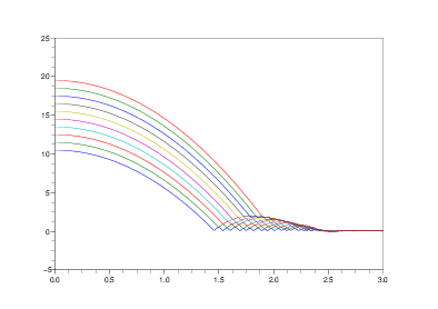
fig 2: Result of MultiBeads simulation#