Simulation of an electrical oscillator supplying a resistor through a half-wave rectifier#

Author: Pascal Denoyelle, September 22, 2005

You may refer to the source code of this example, found here.

There is also a PDF version of this document, viewable online here.

Description of the physical problem : electrical oscillator with half-wave rectifier#

In this sample, a LC oscillator initialized with a given voltage across the capacitor and a null current through the inductor provides the energy to a load resistance through a half-wave rectifier consisting of an ideal diode (see fig 1: Electrical oscillator with half-wave rectifier).

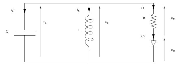
../../_images/SchemaCircuitRLCD.png — fig 1: Electrical oscillator with half-wave rectifier#

Only the positive wave of the oscillating voltage across the LC is provided to the resistor. The energy is dissipated in the resistor resulting in a damped oscillation.

Definition of a general abstract class of NSDS : the linear time invariant complementarity system (LCS)#

This type of non-smooth dynamical system consists of :

a time invariant linear dynamical system (the oscillator). The state variable of this system is denoted by $x$ .
a non-smooth law describing the behaviour of the diode as a complementarity condition between current and reverse voltage (variables ( $y, λ$ ) )
a linear time invariant relation between the state variable $x$ and the non-smooth law variables ( $y, λ$ )

Dynamical system and Boundary conditions#

Remark:

In a more general setting, the system’s evolution would be described by a DAE :

$G \cdot x^{'} = A \cdot x + E \cdot u + b + r$

with $G, A, E$ matrices constant over time (time invariant system), $u, b$ source terms functions of time and $r$ , a term coming from the non-smooth law variables : $r = B \cdot λ + a$ with $B, a$ constant over time. We will consider here the case of an ordinary differential equation :

$x^{'} = A \cdot x + E \cdot u + b + r$

and an initial value problem for which the boundary conditions are $t_{0} \in R, x (t_{0}) = x_{0}$ .

Relation between constrained variables and state variables#

In the linear time invariant framework, the non-smooth law acts on the linear dynamical system evolution through the variable $r = B \cdot λ + a$ . Reciprocally, the state variable $x$ acts on the non-smooth law through the relation $y = C \cdot x + D \cdot λ + F \cdot u + e$ with $C, D, F, e$ constant over time.

Definition of the Non Smooth Law between constrained variables#

It is a complementarity condition between y and $λ$ : $0 \leq y ⊥ λ \geq 0$ . This corresponds to the behaviour of the rectifying diode, as described in Non Smooth laws.

The formalization of the electrical oscillator with half-wave rectifier into the LCS#

The equations come from the following physical laws :

the Kirchhoff current law (KCL) establishes that the sum of the currents arriving at a node is zero,
the Kirchhoff voltage law (KVL) establishes that the sum of the voltage drops in a loop is zero,
the branch constitutive equations define the relation between the current through a bipolar device and the voltage across it

Refering to fig 1: Electrical oscillator with half-wave rectifier, the Kirchhoff laws could be written as:

\begin{array}{r} \begin{array}{l} v_{L} = v_{C} \\ v_{R} + v_{D} = v_{C} \\ i_{C} + i_{L} + i_{R} = 0 \\ i_{R} = i_{D} \end{array} \end{array}

while the branch constitutive equations for linear devices are:

\begin{array}{r} \begin{array}{l} i_{C} = C v_{C}^{'} \\ v_{L} = L i_{L}^{'} \\ v_{R} = R i_{R} \end{array} \end{array}

and last the “branch constitutive equation” of the ideal diode that is no more an equation but instead a complementarity condition:

0 \leq i_{D} ⊥ - v_{D} \geq 0

This is illustrated in fig 2: Non-smooth and smooth characteristics of a diode, where the left-hand sketch displays the ideal diode characteristic and the right-hand sketch displays the usual exponential characteristic as stated by Shockley’s law.

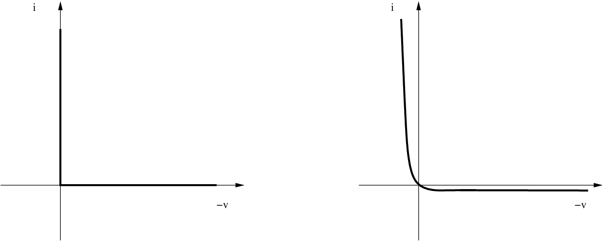
../../_images/diode-caract.png — fig 2: Non-smooth and smooth characteristics of a diode#

Dynamical equation#

After rearranging the previous equations, we obtain:

\begin{array}{r} (\begin{array}{c} v_{L}^{'} \\ i_{L}^{'} \end{array}) = (\begin{array}{cc} 0 & \frac{- 1}{C} \\ \frac{1}{L} & 0 \end{array}) \cdot (\begin{array}{c} v_{L} \\ i_{L} \end{array}) + (\begin{array}{c} \frac{- 1}{C} \\ 0 \end{array}) \cdot i_{D} \end{array}

that fits in the frame of ref{sec-def-NSDS} with

\begin{array}{r} x = (\begin{array}{c} v_{L} \\ i_{L} \end{array}) \end{array}

and

λ = i_{D}

Relations#

We recall that the $r = B \cdot λ + a$ equation is expressed with

\begin{array}{r} r = (\begin{array}{c} \frac{- 1}{C} \\ 0 \end{array}) \cdot i_{D} \end{array}

from the dynamical equation (Dynamical equation).

Rearranging the initial set of equations yields:

\begin{array}{r} - v_{D} = (\begin{array}{cc} - 1 & 0 \end{array}) \cdot (\begin{array}{c} v_{L} \\ i_{L} \end{array}) + R i_{D} \end{array}

as the second equation of the linear time invariant relation with

y = - v_{D}

Non Smooth laws#

There is just the complementarity condition resulting from the ideal diode characteristic:

0 \leq i_{D} ⊥ - v_{D} \geq 0

Description of the numerical simulation: the Moreau’s time-stepping scheme#

Time discretization of the dynamical system#

The integration of the ODE over a time step $[t_{i}, t_{i + 1}]$ of length $h$ is:

\int_{t_{i}}^{t_{i + 1}} x^{'} d t = \int_{t_{i}}^{t_{i + 1}} A \cdot x d t + \int_{t_{i}}^{t_{i + 1}} (E \cdot u + b) d t + \int_{t_{i}}^{t_{i + 1}} r d t

The left-hand term is $x (t_{i + 1}) - x (t_{i})$ .

Right-hand terms are approximated this way:

$\int_{t_{i}}^{t_{i + 1}} A \cdot x d t$ is approximated using a $θ$ -method

$\int_{t_{i}}^{t_{i + 1}} A \cdot x d t \approx h θ (A \cdot x (t_{i + 1})) + h (1 - θ) (A \cdot x (t_{i}))$
since the second integral comes from independent sources, it can be evaluated with whatever quadrature method, for instance a $θ$ -method

$\int_{t_{i}}^{t_{i + 1}} (E \cdot u + b) d t \approx h θ (E \cdot u (t_{i + 1}) + b (t_{i + 1})) + h (1 - θ) (E \cdot u (t_{i}) + b (t_{i}))$
the third integral is approximated like in an implicit Euler integration

$\int_{t_{i}}^{t_{i + 1}} r d t \approx h r (t_{i + 1})$

By replacing the accurate solution $x (t_{i})$ by the approximated value $x_{i}$ , we get:

x_{i + 1} - x_{i} = h θ (A \cdot x_{i + 1}) + h (1 - θ) (A \cdot x_{i}) + h θ (E \cdot u (t_{i + 1}) + b (t_{i + 1})) + h (1 - θ) (E \cdot u (t_{i}) + b (t_{i})) + h r_{i + 1}

Assuming that $I - h θ A$ is invertible, matrix $W$ is defined as $(I - h θ A)^{- 1}$ . We get then:

x_{i + 1} = W (I + h (1 - θ) A) \cdot x_{i} + W (h θ (E \cdot u (t_{i + 1}) + b (t_{i + 1})) + h (1 - θ) (E \cdot u (t_{i}) + b (t_{i}))) + h W r_{i + 1}

An intermediate variable $x_{f r e e}$ related to the smooth part of the system is defined as:

x_{f r e e} = W (I + h (1 - θ) A) \cdot x_{i} + W (h θ (E \cdot u (t_{i + 1}) + b (t_{i + 1})) + h (1 - θ) (E \cdot u (t_{i}) + b (t_{i})))

Thus the calculus of $x_{i + 1}$ becomes:

x_{i + 1} = x_{f r e e} + h W r_{i + 1}

Time discretization of the relations#

It comes straightforwardly:

\begin{array}{r} \begin{aligned} r_{i + 1} = & B \cdot λ_{i + 1} + a \\ y_{i + 1} = & C \cdot x_{i + 1} + D \cdot λ_{i + 1} + F \cdot u (t_{i + 1}) + e \end{aligned} \end{array}

Time discretization of the non-smooth law#

It comes straightforwardly:

0 \leq y_{i + 1} ⊥ λ_{i + 1} \geq 0

Summary of the time discretized equations#

These equations are summarized assuming that there is no source term and simplified relations as for the electrical oscillator with half-wave rectifier.

\begin{array}{r} \begin{array}{ccc} W & = & (I - h θ A)^{- 1} \\ x_{f r e e} & = & W (I + h (1 - θ) A) \cdot x_{i} \\ x_{i + 1} & = & x_{f r e e} + h W r_{i + 1} \\ r_{i + 1} & = & B \cdot λ_{i + 1} \\ y_{i + 1} & = & C \cdot x_{i + 1} + D \cdot λ_{i + 1} \\ 0 \leq y_{i + 1} ⊥ λ_{i + 1} \geq 0 \end{array} \end{array}

Numerical simulation#

The integration algorithm with a fixed step is described here :

Algorthm 1: Integration of the electrical oscillator with half-wave rectifier through a fixed Moreau time stepping scheme

Require: $R > 0, L > 0, C > 0$

Require: Time parameters $h, T, t_{0}$ and $θ$ for the integration

Require: Initial value of inductor voltage $v_{L} = x_{0} (0)$

Require: Optional, initial value of inductor current $i_{L} = x_{0} (1)$ (default: 0)

$n_{s t e p} = \frac{T - t_{0}}{h}$

// Dynamical system specification

$A = (\begin{array}{cc} 0 & \frac{- 1}{C} \\ \frac{1}{L} & 0 \end{array})$

// Relation specification

$B = (\begin{matrix} \frac{- 1}{C} \\ 0 \end{matrix})$

$C = (\begin{array}{cc} - 1 & 0 \end{array})$

$D = (R)$

// Construction of time independent operators

Require: $I - h θ A$ invertible $W = (I - h θ A)^{- 1}$ $M = D + h C W B$

// Non-smooth dynamical system integration

for $i = 0$ to $n_{s t e p} - 1$ do

$\begin{array}{r} \begin{aligned} x_{f r e e} = & W (I + h (1 - θ) A) x_{i} & // Computation of x_{f r e e} \\ q = & C \cdot x_{f r e e} & // Formalization of the one step LCP \\ (y_{i + 1}, λ_{i + 1}) = & solveLCP (M, q) & // One step LCP solving \\ x_{i + 1} = & x_{f r e e} + h W B λ_{i + 1} & // Computation of new state \end{aligned} \end{array}$

end for

Comparison with numerical results coming from SPICE models and algorithms#

We have used the SMASH simulator from Dolphin to perform a simulation of this circuit with a smooth model of the diode as given by Shockley’s law , with a classical one step solver (Newton-Raphson) and a choice between backward-Euler and trapezoidal integrators.

Characteristic of the diode in the SPICE model#

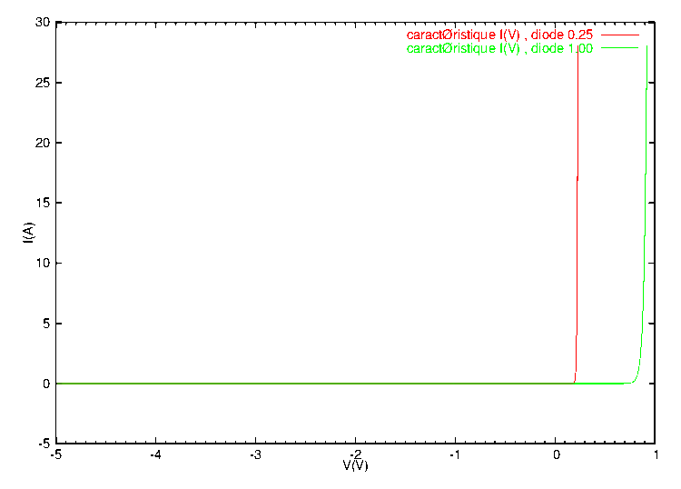
fig 3: Diodes characteristics from SPICE model (N=0.25, N=1) depicts the static $I (V)$ characteristic of two diodes with default SPICE parameters and two values for the emission coefficient $N$ : 1.0 (standard diode) and 0.25 (stiff diode).

../../_images/caracdiode.png — fig 3: Diodes characteristics from SPICE model $(N = 0.25, N = 1)$ #

The stiff diode is close to an ideal one with a threshold of 0.2 V.

Simulation results#

fig 4: SMASH and SICONOS simulation results with backward Euler integration, 10 μs time step displays a comparison of the SMASH and SICONOS results with a backward Euler integration and a fixed time step of 10 μs. A stiff diode model was used in SMASH simulations. For fig 5: SMASH and SICONOS simulation results with trapezoidal integration, 10 μs time step, a trapezoidal integrator was used, yielding a better accuracy. One can notice that the results from both simulators are very close. The slight differences are due to the smooth model of the diode used by SMASH, and mainly to the threshold of around 0.2 V. Such a threshold yields small differences in the conduction state of the diode with respect to the ideal diode.

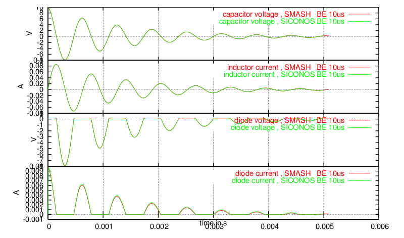
../../_images/comp_SMASH_SICONOS_BE10us.png — fig 4: SMASH and SICONOS simulation results with backward Euler integration, 10 μs time step#

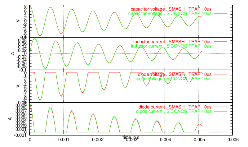
../../_images/comp_SMASH_SICONOS_TRAP10us.png — fig 5: SMASH and SICONOS simulation results with trapezoidal integration, 10 μs time step#

Simulation of an electrical oscillator supplying a resistor through a half-wave rectifier

Contents