Tutorial: A 4-diodes bridge wave rectifier#
Note
the uptodate version of this tutorial is available as a Python notebook in siconos tutorials repository.
Preamble#
This tutorial is dedicated to the simulation of the system shown on fig 1: Diode bridge below. We will describe the step-by-step building of its modelisation as a nonsmooth dynamical system and its time integration.
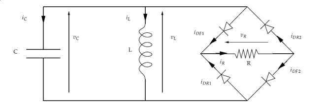
fig 1: Diode bridge#
A LC oscillator initialized with a given voltage across the capacitor and a null current through the inductor provides the energy to a load resistance through a full-wave rectifier consisting of a 4 ideal diodes bridge. Both waves of the oscillating voltage across the LC are provided to the resistor with current flowing always in the same direction. The energy is dissipated in the resistor resulting in a damped oscillation.
The diode behavior is presented on fig 2: diode characteristics, the left-hand sketch displays the ideal diode characteristic and the right-hand sketch displays the usual exponential characteristic as stated by Shockley’s law.
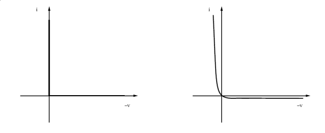
fig 2: diode characteristics#
The diodes, supposed to be ideal, lead to complementarity between voltage and intensity, introducing nonsmoothness into the system. This will be detailed later.
Siconos driver file#
To run a simulation in siconos, it is necessary to write a “driver” file, either in C++ (this file must be compiled and link with siconos libraries) or in python and to execute it. In both cases, the whole process is handled by the ‘siconos’ script:
siconos DiodeBridge.cpp
will compile, link and execute, while:
siconos DiodeBridge.py
will execute your python script.
Siconos can obviously be used in an interactive python session or notebook. This is probably the easiest way to proceed with this tutorial.
Remarks:
this example is available in siconos examples package under Electronics/DiodeBridge directory, in C++, python and as a notebook. For the latter just run:
ipython notebook DiodeBridge.ipynbto interactively run this tutorial.
In this tutorial, we assume that siconos is properly installed on you system, as explained in Build and install.
Let us start with a short description of the three main steps always required to run a simulation.
First of all, you will need to describe properly the system as a nonsmooth dynamical system, i.e. :
define the ordinary differential equations set (the Dynamical Systems) that represent the dynamics,
define the ‘nonsmooth’ part of the system, through nonsmooth laws and relations between variables that may constraint the state.
Then you will need to choose a simulation strategy, to define how the nonsmooth system will be integrated over a time step : which discretisation and integrators for the dynamics (one-step integrators), which formulation and solvers for the nonsmooth problem and so on.
Finally, you will need to run your simulation and post-process the results.
Building a nonsmooth dynamical system#
Modeling the dynamics#
The considered oscillator is a linear dynamical system with time-invariant coefficients. Using the Kirchhoff current and voltage laws and branch constitutive equations, the dynamics of the system writes
and if we denote
we get a first order linear system
with the unknowns \(x\) and \(r\).
To represent this kind of ordinary differential equations, siconos has a class FirstOrderLinearTIDS (TIDS stands for time-invariant coefficients dynamical system)
which inherits from DynamicalSystem. Check Dynamical Systems to find a complete review of all the dynamical systems formalisms available in the software.
# import siconos package
import siconos.kernel as sk
# numpy for vectors and matrices
import numpy as np

# dynamical system parameters
Lvalue = 1e-2    # inductance
Cvalue = 1e-6    # capacitance
Rvalue = 1e3     # resistance
Vinit = 10.0     # initial voltage
x0 = [Vinit, 0.] # initial state
# A matrix of the linear oscillator
A = np.zeros((2, 2), dtype=np.float64)
A.flat[...] = [0., -1.0/Cvalue, 1.0/Lvalue, 0.]

# build the dynamical system
ds = sk.FirstOrderLinearTIDS(x0, A)
A few remarks:
in python you can use either lists or numpy arrays to build vectors or matrices used as siconos methods arguments.
help can be found on siconos objects with the standard python help function. For example, to find how the system can be build:
help(sk.FirstOrderLinearTIDS)
or by checking the siconos_api_reference or siconos_python_reference documention.
Modeling the interactions#
Now, the nonsmooth part of the system must be defined, namely what are the nonsmooth laws and constraints between the variables. In Siconos, the definition of a nonsmooth law and a relation between one or two dynamical systems is called an Interaction (see Interactions between dynamical systems). Thus, the definition of a set of dynamical systems and of interactions between them will lead to the complete nonsmooth dynamical system.
For the oscillator of fig 1: Diode bridge, there exist some linear relations (constraints) between voltage and current inside the diode, given by
with
and recalling that
this is equivalent to the linear relation between \((x, r)\) and \((y, \lambda)\):
To represent this kind of algebraic equations, siconos has a class FirstOrderLinearTIR (TIR stands for time-invariant coefficients relations)
which inherits from Relation. Check Relations to find a complete review of all the relations formalisms available in the software.
# --- build an interaction ---
interaction_size = 4  # number of constraints

# B, C, D matrices of the relation
C = [[0.,   0.],
    [0,    0.],
    [-1.,  0.],
    [1.,   0.]]

D = [[1./Rvalue, 1./Rvalue, -1.,  0.],
    [1./Rvalue, 1./Rvalue,  0., -1.],
    [1.,        0.,         0.,  0.],
    [0.,        1.,         0.,  0.]]

B = [[0.,        0., -1./Cvalue, 1./Cvalue],
    [0.,        0.,  0.,        0.       ]]

# set relation type
relation= sk.FirstOrderLinearTIR(C, B)
relation.setDPtr(D)

# set nonsmooth law
nonsmooth_law = sk.ComplementarityConditionNSL(interaction_size)

# nslaw + relation == interaction
interaction = sk.Interaction(nonsmooth_law, relation)
Notice that a complete FirstOrderLinearTIR writes
All components not set during build are considered to be zero (which is the case here for F and e).
Each diode of the bridge is supposed to be ideal, with the behavior shown on left-hand sketch of fig 2: diode characteristics. Such a behavior can be described with a complementarity condition between current and reverse voltage.
Complementarity between two variables \(y \in R^m, \lambda \in R^m\) writes
or, using “\(\perp\)” symbol,
The inequalities must be considered component-wise.
Then, back to our circuit, the complementarity conditions, results of the ideal diodes characteristics are given by:
with the previously defined \(y\) and \(\lambda\). Note that depending on the diode position in the bridge, \(y_i\) stands for the reverse voltage across the diode or for the diode current.
To represent such a nonsmooth law siconos has a class ComplementarityConditionNSL (you will find NSL in each class-name defining a nonsmooth law)
which inherits from NonSmoothLaw. Check Non Smooth Laws to find a complete review of all available laws in the software.
nonsmooth_law = sk.ComplementarityConditionNSL(interaction_size)
The interaction can be completely defined:
interaction = sk.Interaction(nonsmooth_law, relation)
Notice that this interaction just describe some relations and laws but is not connected to any real dynamical system, for the moment.
The modeling part is almost complete, since only one dynamical system and one interaction are needed to describe the problem.
They must be gathered into a specific object, the NonSmoothDynamicalSystem.
The building of this object is quite simple: just
set the time window for the simulation, include dynamical systems and link them to the correct interactions.
# dynamical systems and interactions must be gathered into a NonSmoothDynamicalSystem
t0 = 0. # initial time
T = 5.0e-3 # duration of the simulation
DiodeBridge = sk.NonSmoothDynamicalSystem(t0, T)
# add the dynamical system in the non smooth dynamical system
DiodeBridge.insertDynamicalSystem(ds)

# link the interaction and the dynamical system
DiodeBridge.link(interaction, ds)
Describing the simulation of the nonsmooth dynamical system#
You need now to define how the nonsmooth dynamical system will be integrated over time. This is the role of the simulation, which must set:
how dynamical systems are discretized and integrate over a time step
how the nonsmooth problem will be formalized and solved
Two different strategies are available : event-capturing (a.k.a time stepping) schemes and event-driven schemes. Check Simulation of non-smooth dynamical systems for details or [1] for even more details.
For the Diode Bridge example, an event-capturing strategy will be used, with an Euler-Moreau integrator and a LCP (Linear Complementarity Problem) formulation.
Let us start with the ‘one-step integrator’, i.e. the description of the discretisation and integration of the dynamics over a time step, between time \(t_i\) and \(t_{i+1}\). The integration of the equation over the time step is based on a \(\theta\) -method. The process is detailed in Event-Capturing schemes and, for first-order systems, leads to
This corresponds to EulerMoreauOSI integrators, which inherits from OneStepIntegrator. Check Time integration of the dynamics to find a complete review of integrators available in the software.
theta = 0.5
osi = sk.EulerMoreauOSI(theta)
Notice that each dynamical system of the model must be associated to one and only one one-step integrator.
Next, based on the simulation strategy and the time-integration, a one-step nonsmooth problem must be formalized, see Simulation of non-smooth dynamical systems and Nonsmooth problems formulation and solve.
Considering the following discretization of the previously defined relations and nonsmooth law
we get
with
This is known as a Linear Complementarity Problem, written in siconos thanks to LCP class, which inherits from OneStepNSProblem.
As usual, check Nonsmooth problems formulation and solve for a complete review of the nonsmooth problems formulations available in Siconos.
To each formulation, one must associate a solver, picked from the list given in LCP available solvers:
import siconos.numerics as sn
#  Non smooth problem
osnspb = sk.LCP(sn.SICONOS_LCP_NSQP)
Notice that solvers come from siconos numerics and are identified thanks to an id. The connection between ids and solvers is given in LCP available solvers.
Then the last step consists in the simulation creation, with its time discretisation:
# simulation and time discretisation
time_step =  1.0e-6
td = sk.TimeDiscretisation(t0, time_step)
simu = sk.TimeStepping(DiodeBridge, td, osi, osnspb)
Leading the Simulation Process#
The easiest way to run your simulation is to call:
s->run()
But after that you only have access to values computed at the last time step, which might not be enough …
For the present case, \(x, y \ and \ \lambda\) at each time step are needed for postprocessing. Here is an example on how to get and save them in a numpy array:
N = int((T - t0) / simu.timeStep()) + 1
data_plot = np.zeros((N, 8))
y = interaction.y(0)
lamb = interaction.lambda_(0)
x = ds.x()
k = 0
data_plot[k, 1] = x[0] #  inductor voltage
data_plot[k, 2] = x[1] # inductor current
data_plot[k, 3] = y[0] # diode R1 current
data_plot[k, 4] = - lamb[0] # diode R1 voltage
data_plot[k, 5] = - lamb[1] # diode F2 voltage
data_plot[k, 6] = lamb[2] # diode F1 current
data_plot[k, 7] = y[0] + lamb[2] # resistor current
while simu.hasNextEvent():
    k += 1
    simu.computeOneStep()
    data_plot[k, 0] = simu.nextTime()
    data_plot[k, 1] = x[0]
    data_plot[k, 2] = x[1]
    data_plot[k, 3] = y[0]
    data_plot[k, 4] = - lamb[0]
    data_plot[k, 5] = - lamb[1]
    data_plot[k, 6] = lamb[2]
    data_plot[k, 7] = y[0] + lamb[2]
    simu.nextStep()
Simulation::hasNextEvent()is true as long as there are events to be considered, i.e. until T is reachedSimulation::nextStep()is mainly used to increment the time step, save current state and prepare initial values for next step.Simulation::computeOneStep()performs computation over the current time step. In the Moreau’s time stepping case, it will first integrate the dynamics to obtain the so-called free-state, that is without non-smooth effects, then it will formalize and solve a LCP before re-integrate the dynamics using the LCP results.
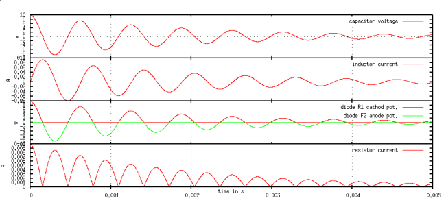
The results can now be postprocessed, with matplotlib for example:
import matplotlib.pyplot as plt
plt.subplot(411)
plt.title('inductor voltage')
plt.plot(data_plot[0:k - 1, 0], data_plot[0:k - 1, 1])
plt.grid()
plt.subplot(412)
plt.title('inductor current')
plt.plot(data_plot[0:k - 1, 0], data_plot[0:k - 1, 2])
plt.grid()
plt.subplot(413)
plt.title('diode R1 (blue) and F2 (green) voltage')
plt.plot(data_plot[0:k - 1, 0], -data_plot[0:k - 1, 4])
plt.plot(data_plot[0:k - 1, 0], data_plot[0:k - 1, 5])
plt.grid()
plt.subplot(414)
plt.title('resistor current')
plt.plot(data_plot[0:k - 1, 0], data_plot[0:k - 1, 7])
plt.grid()